Understanding Traffic Mobility using Computer Vision

The following is an account of one of the projects I worked on during my undergraduate years. It outlines the problem we were trying to solve, the techincal details behind the system we developed and my experience and learning from the project.

With the advent of deep learning, the field that has arguably been hyped the most in the recent years is Computer Vision. The ability to understand the elements and activities in a still image or a moving video presents endless opportunities for digitizing aspects of human life that was not possible previously. One such example is understanding the flow of vehicle traffic in the road solely through surveillance cameras. This is the problem we attempted to tackle as our undergraduate minor thesis.

Problem Statement

The primary task is to build a system for analysing traffic mobility pattern in the roads of Kathmandu, Nepal. Understanding the vehicle traffic in a road entails two primary tasks:

Vehicle Detection, or in general, object detection which further encompasses two sub-tasks:
- Classification: We need to first be able to categorize the vehicle into one of the many categories like bus, cars, taxi, motorbikes, trucks, etc.
- Localization: Simply classifying the vehicles won’t cut it. We should also be able to localize its position in the frame. In other words, we need to identify a bounding box that encloses the vehicle.
Vehicle Tracking: Traffic is ever moving. So we need to be able to track the movement of the vehicles in the road. For this project, we decided to only count the number of vehicles that went past the camera. Measuring their velocity could have been an enhancement.

System Overview

Before diving into the technical details behind the solution we developed, it helps to have a bigger picture of the problem we were attempting to tackle and discuss what an ideal system could look like.

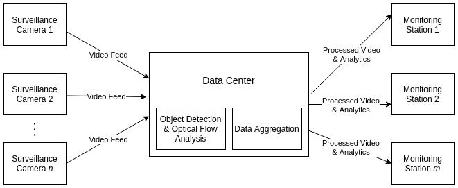
Fig: Block diagram of the expected traffic mobility analysis system.

The system consists of 3 major components:

Surveillance Cameras: The traffic surveillance cameras placed in the road that supply the video feed to the data center.
Data Center: The place where the video data is stored and processed. Specifically, it is here where the detection and tracking of vehicles in the video frame would take place. The resulting data is then aggregated to produce human readable information for analysis.
Monitoring Station: This is the client side of the application where the processed video (with the detected vehicles) are shown along with informative dashboard to help the users make sense of the traffic mobility pattern. It will display the following information:
- The real-time count of the vehicles (categorized by type) in the road
- The plot of amount of road occupancy against time elapsed.

Task 1: Vehicle Detection

Now onto the technical details. If you have anything to do with images (videos are simply a stream of images), Convolutional Neural Networks (CNN) are the de-facto standard in deep learning. Specifically for this task of object detection, we employed YOLOv2 network. YOLO (You Only Look Once) is a CNN architecture that is tailored to detect objects in an image at lightning speed. I will be only surfacely describing the working of this architecture to maintain brevity. For a rigorous technical treatment, please refer to the following papers:

YOLO in Brief

Traditionally, object detection algorithms worked by running classifiers on parts of the image in a sliding window. This was the case for architectures like Faster R-CNN. While they boasted high accuracy, the inference time is too slow to be feasibly used in a real time object detection from video. YOLO transformed the literature by framing object detection as a regression problem. The result is faster inference with small tradeoff in accuracy.

YOLOv2 is an improvement on the older YOLO architecture and is the state of the art in standard detection tasks like PASCAL VOC and COCO. At 67 FPS, YOLOv2 gets 76.2 mAP on VOC 2007 while at 40 FPS, YOLOv2 gets 78.6 mAP. It outperforms Faster R-CNN with ResNet and SSD while still running faster than them.

What does YOLO output?

Fig: YOLO divides the image into [S x S] grid and each grid has B bounding boxes predictions along with their confidence and class probabilities.

YOLO divides the image into a \(S \times S\) grid. Each grid cell has \(B\) bounding box predictions. Each bounding box prediction is represented by a vector of length 5. This vector includes all the information that would need to represent the prediction of a bounding box:

\((x,y)\): The coordinates of the center of the boxes relative to the grid cell.
\((w, h)\): The width and height of the box relative to the entire image.
\(P(obj)\): The confidence score or the probability that there is an object in the box

Now, the object (if present) in the grid cell could belong to any of the \(k\) classes. Each grid cell also predicts class conditional probabilities vector \(C = \begin{bmatrix} C_1 & C_2 & \dots & C_k \end{bmatrix}\) where \(C_i = P(Class_i \| Object )\). Consequently, \(P(obj) * C_i\) gives the probability that an object of class \(C_i\) exists in the box.

The concept of Anchor Boxes

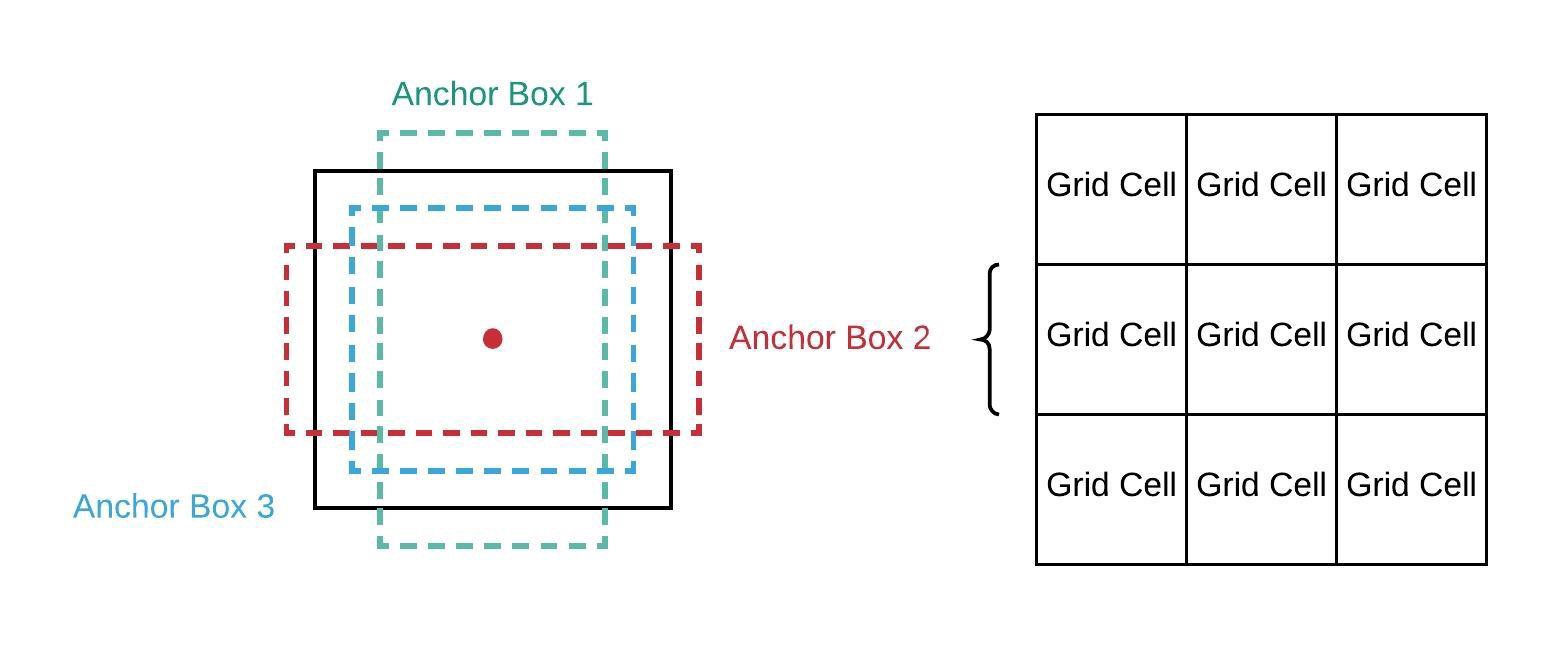
Fig: Different shapes of anchor boxes in a grid cell

A square bounding box is not always the best choice for different shapes of objects we might need to detect. For instance, trees are better demarcated by vertical rectangles while a car might need horizontal rectangles. YOLOv2 uses anchor boxes as a solution which differentiates and improves it from its predecessor. Anchor boxes are set of boxes with predefined width/height ratio. Instead of directly predicting the bounding box coordinate, we then predict the offsets for these boxes such that it will enclose an object. Now, you might be wondering how does YOLO identify the best choice among these boxes. For this, it uses a concept called Intersection Over Union (IOU). This is the extent of overlap between the predicted bounding box and the ground truth bounding box. Its value is in the range \([0,1]\).

Effectively, for each box, we can calculate:

\[P(obj) * C_i * IoU\]

which gives the probability of an object of a particular class appearing inside that box and how preicse those box co-ordinates are in demarcating the object

The Network Architecture

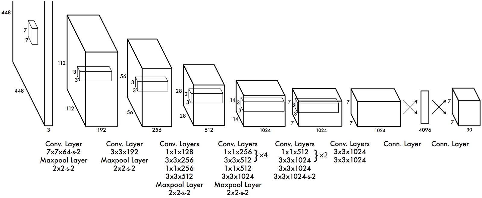
The architecture of YOLOv1 consists of elements what you’d typically see in a CNN architecture. It has a series of convolution layers with maxpool layers in between them. YOLOv2 architecture has slight modifications to the architecture presented above. Notably:

It includes Batch Normalization layers that normalizes the hidden layers which is proven to make the network train faster and also to decrease the internal covariate shift.
It omits the fully connected layers at the end to use anchor boxes instead. The output feature map is \(13 \times 13\)

Loss Function

Now let’s discuss how the model learns. In other words, what loss function does the network use to correct its erroneous predictions and learn to detect objects with greater accuracy. The prediction of a YOLO network can be divided into 3 groups:

\([ x, y, w, h ]\) for localization.
\(P(obj)\) that gives the confidence score on whether an object is present
\(C\) which denote the possibility of presence of each class.

Loss is calculated separately for each and combined together:

Localization Loss:
- Sum of squares of errors for \((x,y)\) and \((w,h)\). The loss is configured to penalize only those boxes that have the highest IOU.
Confidence Loss:
- This is also a SSE loss and it is upweighted for boxes that contain an object whereas it is downweighted for objects that do not contain an object.
Classification Loss:
- This is also a SSE loss to capture the errors in predicting the class conditional probabilities.

The mathematical formulation of the loss function is quite involved and I would suggest the interested reader to check out the original paper for a detailed description.

The nuances in dealing with Nepali vehicles

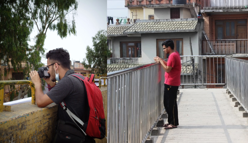
A machine learning model is only as good as its data. In other words, we cannot expect the model to perform well on data that are not representative of the data present in the training dataset. We experienced this problem first hand as the vehicles in Nepal are quite different from what you’d see in western countries. For instance, western countries have far less motorbikes in the road, whereas Nepal has 10 motorbikes for every car in the road. Similarly, the buses, trucks and taxis are quite different in appearance. While the standard ImageNet and COCO dataset have images of standard vehicles, we needed a dataset of Nepali vehicles.

Fig: The 8 types of vehicles detected by our system. Notice how different the vehicles look from vehicles in common vehicle datasets

We captured footages of vehicles in the roads of major intersection of Kathmandu city and collected and annotated a dataset consisting of 10,000 images. The vehicles were categorized into the following 8 classes:

Taxi, Tempo, Motorbike, Car, Microbus, Pickup Truck, Truck, Bus

Fig: Men in action collecting the pictures of Nepali vehicles in roads of Kathmandu

Task 2: Vehicle Tracking

Having figured out a way to classify and localize vehicles in the frames of the video, the next task in hand was to track the individual vehicles in the frame. We need to do this to count the total number of vehicles that moved past the surveillance camera. This will ultimately help us calculate the extent of road occupancy and thereby provide a real time traffic monitoring capability to the end user.

Moving objects are tracked by a technique called Optical Flow. We implemented Lucas-Kanade Optical Flow Algorithm in OpenCV to track the moving vehicles in the road.

Optical Flow

Optical Flow is the apparent motion of objects, surfaces or edges based on the relative motion of the camera.

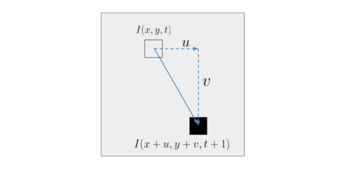
Fig: Movement of a pixel from one point to another across time

The above picture shows a pixel that moved from the point \((x,y)\) at time \(t\) to a new point \((x + u, y + v)\) in time \((t+1)\). \(I(x,y,t)\) represents the brightness or intensity of the pixel at position and time \((x,y,t)\) and \(I(x+u, y+v, t+1)\) is the intensity or brightness of the pixel at new position and time \((x+u, y+v, t+1)\)

Given the position of the pixel in two frames of a video, it would be fairly easy to calculate the velocity and hence track the movement of the vehicle in the video. We already have the bounding boxes given by YOLO. All we need to do is track the centre of this bounding box for each vehicle. Right?

Well, the problem here is that we cannot associate a pixel in the frame \(t+1\) to the pixel in the frame \(t\) such that both the pixel represent the same object. Optical flow aims to solve this problem by making 2 assumptions:

The movement of the pixel is small such that the “moved” pixel in the frame 2 lies within the neighborhood of pixel in frame 1.
The intensity of the pixel doesn’t change from frame 1 to frame 2 and from position 1 to position 2. Atleast not by much.

Mathematically representing,

\[\begin{equation} \frac{\partial I}{\partial t} + \frac{\partial I}{\partial x} . u + \frac{\partial I}{\partial y} . v = 0 \end{equation}\]

Simplifying the notation,

\[\begin{equation} I_t . 1 + I_x . u + I_y . v = 0 \end{equation}\]

The above system of equations cannot be solved as it has 2 unknowns and only 1 equation. Hence, we make another assumption, i.e. a bunch of pixels within a neighborhood move with the same velocities \((u,v)\) from \(t\) to \(t+1\). This gives us a number of equations similar to the one above and we can devise a solution for \((u,v)\) using least squares method.

\[\begin{equation} \begin{bmatrix} I_{t_1} \\ I_{t_2} \\ \vdots \\ I_{t_n} \end{bmatrix} + \begin{bmatrix} I_{x_1} && I_{y_1} \\ I_{x_2} && I_{y_2} \\ \vdots && \vdots \\ I_{x_n} && I_{y_n} \end{bmatrix} . \begin{bmatrix} u \\ v \end{bmatrix} = 0 \end{equation}\] \[\begin{equation} -B + A.X = 0 \end{equation}\] \[\begin{equation} X = (A^TA)^{-1}A^TB \end{equation}\]

We used the centre of the bounding boxes given by YOLO as the points that is tracked. The above algorithm predicts the most probable location a particular point will reach in the next frame and this information is used to track the vehicles movement throughout the video.

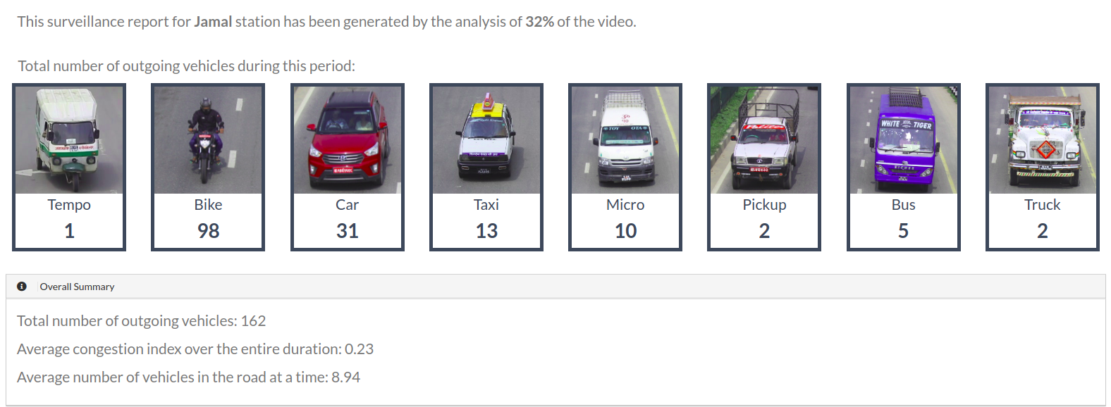
Final Result

Finally, we had the system in place which performed the two most important tasks:

Detecting the vehicles in the road
Tracking the movement of a vehicle throughout the screen

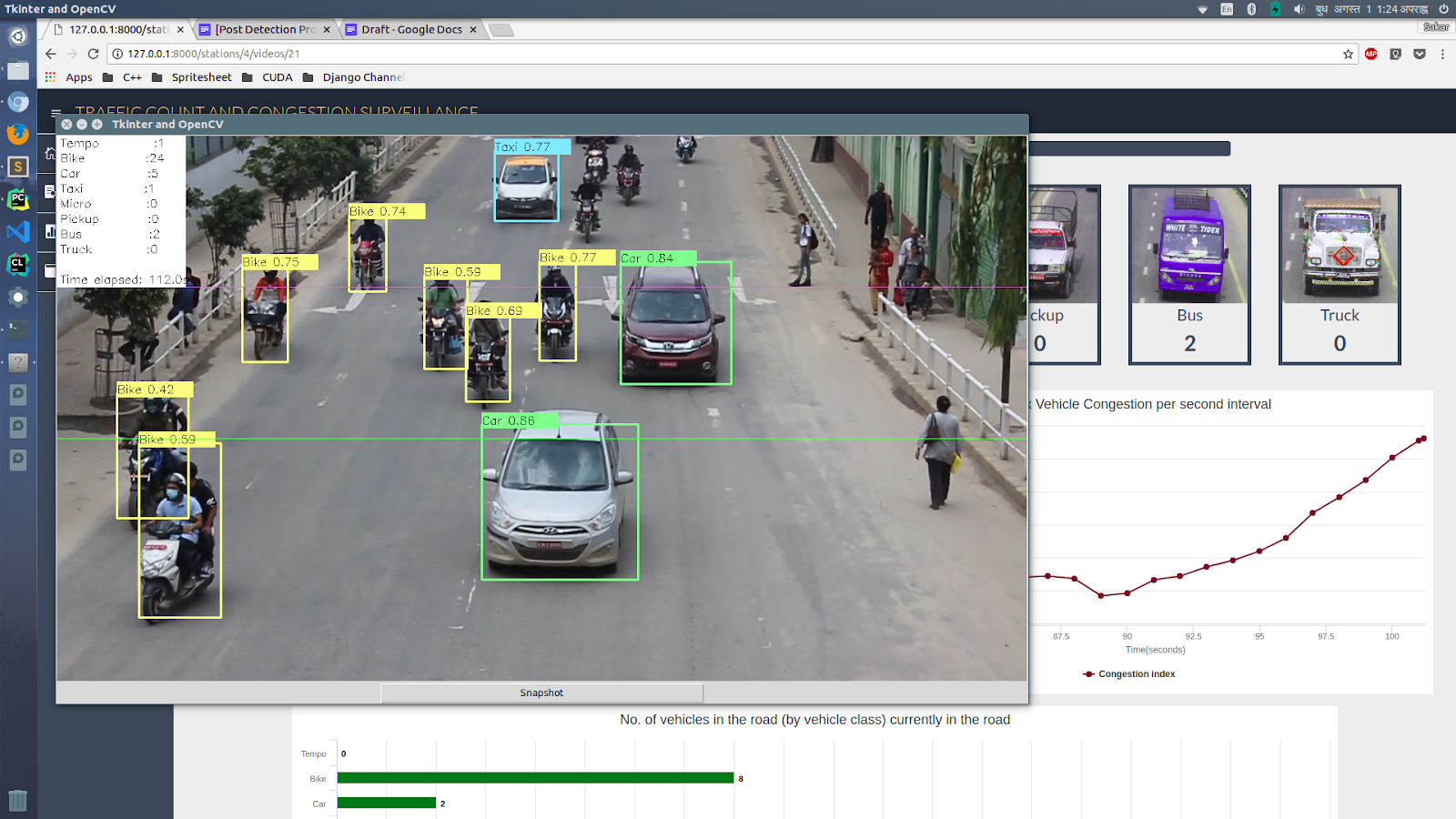
Now, we developed an analytics dashboard for the monitoring station that gave information relevant to the traffic mobility of any road. Some of the details presented in the dashboard were:

The total count of vehicle categorized by its type
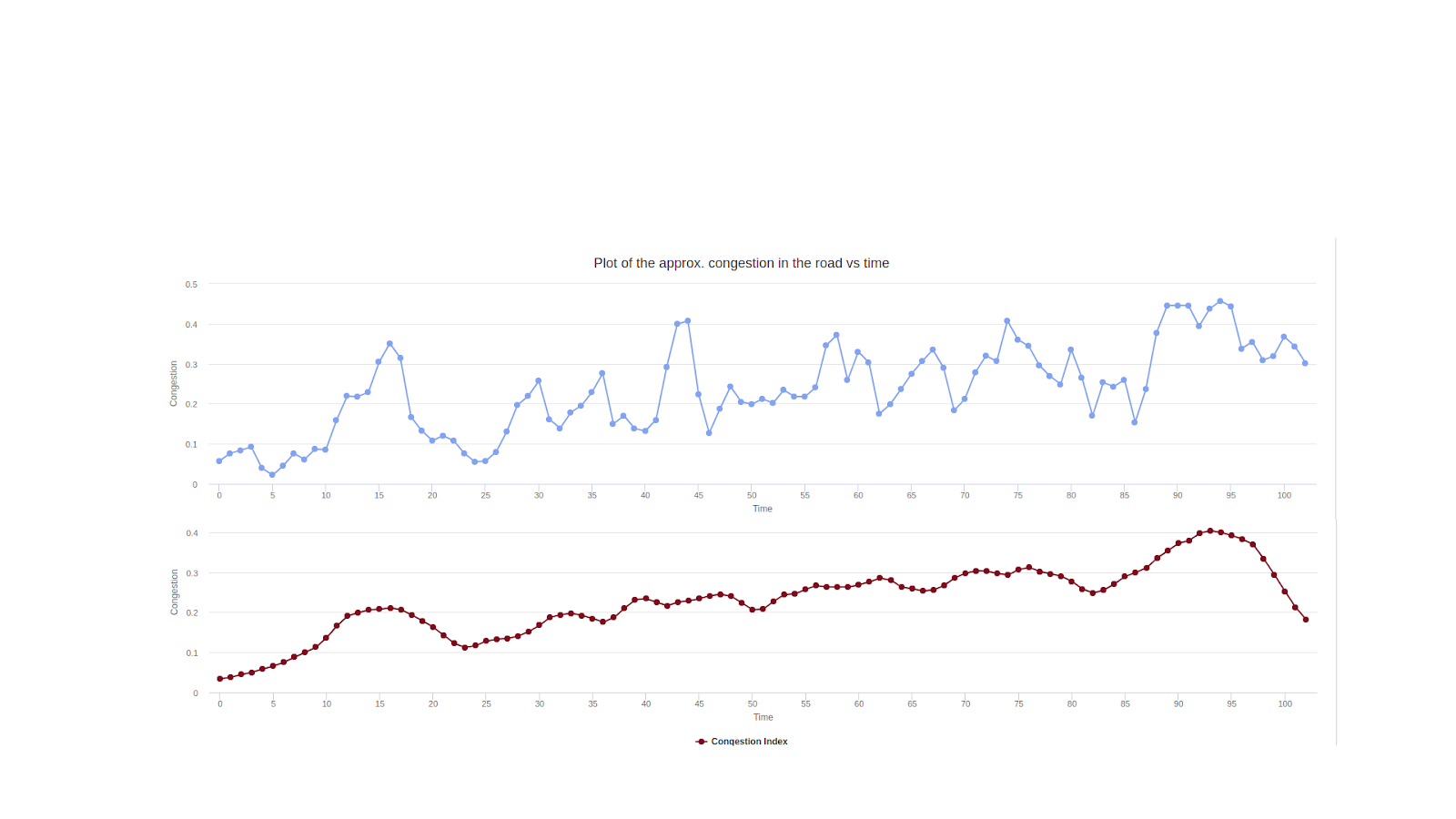
The extent of road occupancy. In other words, how congested the road looks at a particular time.
Identify which periods in a day are the busiest. Vehicle count and road occupancy were taken into consideration for this.

Fig: The dashboard in the monitoring station that displays the real time feed of the road augmented with mobility analytics.

Learnings and Experiences

This was a tranformative project for me. It helped me sink my teeth into the field of computer vision and especially helped me realize how challenging is it to collect and prepare a custom dataset and fine tune a model to perform as expected.

We demonstrated this project to the Metropolitan Traffic Division at Kathmandu and it was well received.

We also won the Smart Urban Technology Challenge 2018 with this very project.

All in all, it was a wonderful experience taking this project from idea to implementation.

Understanding Traffic Mobility using Computer Vision

Categories

Tags